python numpy

What is a Python NumPy?

NumPy is a Python package which stands for ‘Numerical Python’. It is the core library for scientific computing, which contains a powerful n-dimensional array object, provide tools for integrating C, C++ etc. It is also useful in linear algebra, random number capability etc. NumPy array can also be used as an efficient multi-dimensional container for generic data. Now, let me tell you what exactly is a python numpy array.

NumPy Array: Numpy array is a powerful N-dimensional array object which is in the form of rows and columns. We can initialize numpy arrays from nested Python lists and access it elements. In order to perform these numpy operations, the next question which will come in your mind is:

How do I install NumPy?

To install Python NumPy, go to your command prompt and type “pip install numpy”.

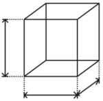
Here, I have different elements that are stored in their respective memory locations. It is said to be two dimensional because it has rows as well as columns. In the above image, we have 3 columns and 4 rows available.

Let us see how it is implemented in PyCharm:

Single-dimensional Numpy Array:

1 2 3

from numpy import * a=array([1,2,3]) print(a)

Output – [1 2 3]

Multi-dimensional Array:

1 2	a=array([(1,2,3),(4,5,6)]) print(a)

O/P – [[ 1 2 3]
[4 5 6]]

Many of you must be wondering that why do we use python numpy if we already have python list? So, let us understand with some examples in this python numpy tutorial.

Python NumPy Array v/s List

We use python numpy array instead of a list because of the below three reasons:

1. Less Memory
2. Fast
3. Convenient

The very first reason to choose python numpy array is that it occupies less memory as compared to list. Then, it is pretty fast in terms of execution and at the same time it is very convenient to work with numpy. So these are the major advantages that python numpy array has over list.

Python NumPy Operations

• ndim:
  You can find the dimension of the array, whether it is a two-dimensional array or a single dimensional array. So, let us see this practically how we can find the dimensions. In the below code, with the help of ‘ndim’ function, I can find whether the array is of single dimension or multi dimension.

1 2 3

from numpy import * a = array([(1,2,3),(4,5,6)]) print(a.ndim)

Output – 2
Since the output is 2, it is a two-dimensional array (multi dimension).

• itemsize:
  You can calculate the byte size of each element. In the below code, I have defined a single dimensional array and with the help of ‘itemsize’ function, we can find the size of each element.

  1 2 3

  from numpy import * a = array([(1,2,3)]) print(a.itemsize)

  Output – 4
  So every element occupies 4 byte in the above numpy array.
• dtype:
  You can find the data type of the elements that are stored in an array. So, if you want to know the data type of a particular element, you can use ‘dtype’ function which will print the datatype along with the size. In the below code, I have defined an array where I have used the same function.

1 2 3

from numpy import * a = array([(1,2,3)]) print(a.dtype)

Output – int32

As you can see, the data type of the array is integer 32 bits. Similarly, you can find the size and shape of the array using ‘size’ and ‘shape’ function respectively.

Output – 6 (1,6)

Next, let us move forward and see what are the other operations that you can perform with python numpy module. We can also perform reshape as well as slicing operation using python numpy operation. But, what exactly is reshape and slicing? So let me explain this one by one in this python numpy tutorial.

• reshape:
  Reshape is when you change the number of rows and columns which gives a new view to an object. Now, let us take an example to reshape the below array:
   
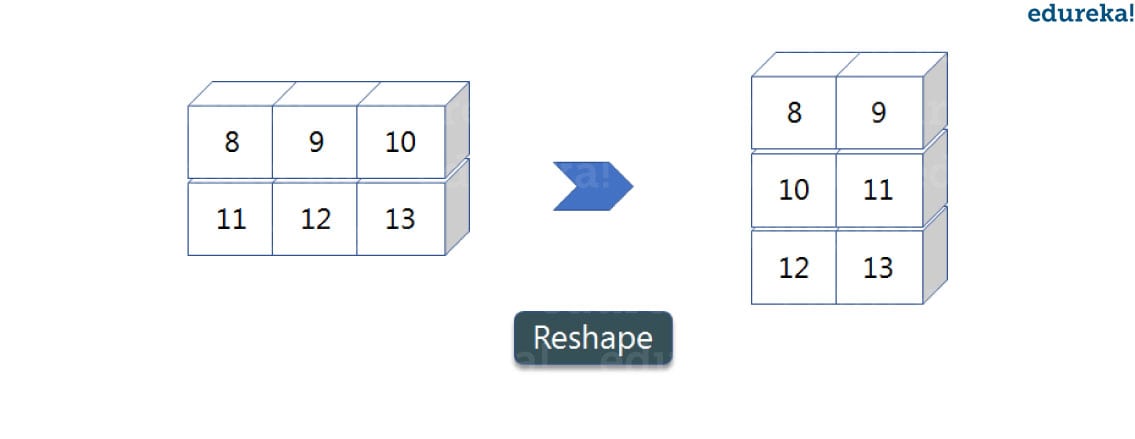
  As you can see in the above image, we have 3 columns and 2 rows which has converted into 2 columns and 3 rows. Let me show you practically how it’s done.

  1 2 3 4 5

  from numpy import * a = array([(8,9,10),(11,12,13)]) print(a) a=a.reshape(3,2) print(a)

  Output – [[ 8 9 10] [11 12 13]] [[ 8 9] [10 11] [12 13]]
• slicing:
  As you can see the ‘reshape’ function has showed its magic. Now, let’s take another operation i.e Slicing. Slicing is basically extracting particular set of elements from an array. This slicing operation is pretty much similar to the one which is there in the list as well. Consider the following example:
  
  Before getting into the above example, let’s see a simple one. We have an array and we need a particular element (say 3) out of a given array. Let’s consider the below example:

  1 2 3

  import numpy as np a=np.array([(1,2,3,4),(3,4,5,6)]) print(a[0,2])

  Output – 3
  
  Here, the array(1,2,3,4) is your index 0 and (3,4,5,6) is index 1 of the python numpy array. Therefore, we have printed the second element from the zeroth index.
  Taking one step forward, let’s say we need the 2nd element from the zeroth and first index of the array. Let’s see how you can perform this operation:

  1 2 3

  import numpy as np a=np.array([(1,2,3,4),(3,4,5,6)]) print(a[0:,2])

  Output – [3 5]
  
  Here colon represents all the rows, including zero. Now to get the 2nd element, we’ll call index 2 from both of the rows which gives us the value 3 and 5 respectively.
  Next, just to remove the confusion, let’s say we have one more row and we don’t want to get its 2nd element printed just as the image above. What we can do in such case?
  Consider the below code:

  1 2 3

  import numpy as np a=np.array([(8,9),(10,11),(12,13)]) print(a[0:2,1])

  Output – [9 11]
  
  As you can see in the above code, only 9 and 11 gets printed. Now when I have written 0:2, this does not include the second index of the third row of an array. Therefore, only 9 and 11 gets printed else you will get all the elements i.e [9 11 13].
• linspace
  This is another operation in python numpy which returns evenly spaced numbers over a specified interval. Consider the below example:

  1 2 3

  import numpy as np a=np.linspace(1,3,10) print(a)

  Output – [ 1. 1.22222222 1.44444444 1.66666667 1.88888889 2.11111111 2.33333333 2.55555556 2.77777778 3. ]
  
  As you can see in the result, it has printed 10 values between 1 to 3.
• max/ min
  Next, we have some more operations in numpy such as to find the minimum, maximum as well the sum of the numpy array. Let’s go ahead in python numpy tutorial and execute it practically.

  1 2 3 4 5 6

  import numpy as np a= np.array([1,2,3]) print(a.min()) print(a.max()) print(a.sum())

  Output – 1 3 6
  
  You must be finding these pretty basic, but with the help of this knowledge you can perform a lot bigger tasks as well. Now, lets understand the concept of axis in python numpy.
  
  
  
  
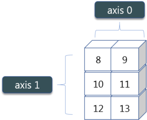
  As you can see in the figure, we have a numpy array 2*3. Here the rows are called as axis 1 and the columns are called as axis 0. Now you must be wondering what is the use of these axis?
  Suppose you want to calculate the sum of all the columns, then you can make use of axis. Let me show you practically, how you can implement axis in your PyCharm:

  1 2	a= np.array([(1,2,3),(3,4,5)]) print(a.sum(axis=0))

  Output – [4 6 8]
  
  Therefore, the sum of all the columns are added where 1+3=4, 2+4=6 and 3+5=8. Similarly, if you replace the axis by 1, then it will print [6 12] where all the rows get added.
• Square Root & Standard Deviation
  There are various mathematical functions that can be performed using python numpy. You can find the square root, standard deviation of the array. So, let’s implement these operations:
  

  1 2 3 4

  import numpy as np a=np.array([(1,2,3),(3,4,5,)]) print(np.sqrt(a)) print(np.std(a))

  Output – [[ 1. 1.41421356 1.73205081]
  [ 1.73205081 2. 2.23606798]]
  1.29099444874
  
  
  As you can see the output above, the square root of all the elements are printed. Also, the standard deviation is printed for the above array i.e how much each element varies from the mean value of the python numpy array.
• Addition Operation
  
  You can perform more operations on numpy array i.e addition, subtraction,multiplication and division of the two matrices. Let me go ahead in python numpy tutorial, and show it to you practically: 

  1 2 3 4

  import numpy as np x= np.array([(1,2,3),(3,4,5)]) y= np.array([(1,2,3),(3,4,5)]) print(x+y)

  Output – [[ 2 4 6] [ 6 8 10]]
  
  This is extremely simple! Right? Similarly, we can perform other operations such as subtraction, multiplication and division. Consider the below example:

  1 2 3 4 5 6

  import numpy as np x= np.array([(1,2,3),(3,4,5)]) y= np.array([(1,2,3),(3,4,5)]) print(x-y) print(x*y) print(x/y)

  Output – [[0 0 0] [0 0 0]]
  [[ 1 4 9] [ 9 16 25]]
  [[ 1. 1. 1.] [ 1. 1. 1.]]
• Vertical & Horizontal Stacking
  Next, if you want to concatenate two arrays and not just add them, you can perform it using two ways – vertical stacking and horizontal stacking. Let me show it one by one in this python numpy tutorial.

  1 2 3 4 5

  import numpy as np x= np.array([(1,2,3),(3,4,5)]) y= np.array([(1,2,3),(3,4,5)]) print(np.vstack((x,y))) print(np.hstack((x,y)))

  Output – [[1 2 3] [3 4 5] [1 2 3] [3 4 5]]
  [[1 2 3 1 2 3] [3 4 5 3 4 5]]

 

python tutorial

http://www.tutorialspoint.com/python3/python_tutorial.pdf?fbclid=IwAR1eiiOIUuzFmtkIsMqNB0iJgF5v9c4eGNY3QTMrFyR_-xfxv7P8XFM4syU

python hands on exercises

Hands on Exercises

Basic Programs:

1.      Program to print ASCII Value of a character

2.      Python Program to Read a Number n and Compute  n+nn+nnn

3.      Python program to display calendar of given month of the year

4.      Python Program to check Armstrong Number

5.      Python program to print all Prime numbers in an Interval

6.      Python Program for Fibonacci numbers

7.      Python Program for Sum of squares of first n natural numbers

Array Programs:

1.      Python Program to find sum of array

2.      Python Program to find largest element in an array

3.      Python Program for array rotation

4.      Python Program for Reversal algorithm for array rotation

5.      Python Program to Split the array and add the first part to the end

6.      Python Program to check if given array is Monotonic

   7.    Write a python program to read a number and print a matrix of n*n size in spiral order with row sums and column sum and diagonal elements sum?

Hint: n=4 then print 4*4 matrix should be like

List Programs:

1.      Python program to interchange first and last elements in a list

2.      Python | Ways to check if element exists in list

3.      Python | Reversing a List

4.      Python | Count occurrences of an element in a list

5.      Python program to find sum of elements in list

6.      Python program to find second largest number in a list

7.      Python program to count Even and Odd numbers in a List

8.      Python | Program to print duplicates from a list of integers

String Programs:

1.      Python program to check if a string is palindrome or not

2.      Print the substring “WELCOME” from the given string “WELCOME TO PYTHON LANGUAGE”

3.      Reverse words in a given String in Python

4.      Ways to remove given character from string in Python

5.      Python | Check if a Substring is Present in a Given String

6.      Remove all duplicates from a given string in Python

7.      Python program to split and join a string

Tuple Programs:

1.      Create a list of tuples from given list having number and its cube in each tuple

2.      Sort a list of tuples by second Item

Dictionary Programs:

1.      Python | Find largest value and key in  Dictionarie e

2.      Handling missing keys in Python dictionaries

3.      Python program to find the sum of all items in a dictionary

4.      Python | Ways to remove a key from dictionary

5.      Python | Merging two Dictionaries

6.      Dictionary and counter in Python to find winner of election

7.      Counting the frequencies in a list using dictionary in Python

Sets programs

1.      Python Program to Count the Number of Vowels Present in a String using Sets

2.      Python Program to Check Common Letters in Two Input Strings

3.       Python Program that Displays which Letters are in the First String but not in the Second

File Handling Programs:

1.      Python Program to Count the Number of Lines in a Text File

2.      Python Program to Read a String from the User and Append it into a File

3.      Python Program to Count the Occurrences of a Word in a Text File

4.      Python Program to Copy the Contents of One File into Another

5.      Python Program to Append the Contents of One File to Another File

6.      Python Program to Count the Number of Blank Spaces in a Text File

7.      Write a python program to create a file with roll no, name, year, sem and 6 subject marks and write them in a file and then calculate the total, percentage of each student and also find the rank of each student in the file?

python basics

span>Preliminaries
1.1 What is Python?
Python is a powerful modern computer programming language. It bears some similarities to
Fortran, one of the earliest programming languages, but it is much more powerful than Fortran.
Python allows you to use variables without declaring them (i.e., it determines types implicitly),
and it relies on indentation as a control structure. You are not forced to define classes in Python
(unlike Java) but you are free to do so when convenient.
Python was developed by Guido van Rossum, and it is free software. Free as in “free beer,” in that
you can obtain Python without spending any money. But Python is also free in other important
ways, for example you are free to copy it as many times as you like, and free to study the source
code, and make changes to it. There is a worldwide movement behind the idea of free software,
initiated in 1983 by Richard Stallman.1
This document focuses on learning Python for the purpose of doing mathematical calculations.
We assume the reader has some knowledge of basic mathematics, but we try not to assume any
previous exposure to computer programming, although some such exposure would certainly be
helpful. Python is a good choice for mathematical calculations, since we can write code quickly, test
it easily, and its syntax is similar to the way mathematical ideas are expressed in the mathematical
literature. By learning Python you will also be learning a major tool used by many web developers.
1.2 Installation and documentation
If you use Mac OS X or Linux, then Python should already be installed on your computer by
default. If not, you can download the latest version by visiting the Python home page, at
http://www.python.org
where you will also find loads of documentation and other useful information. Windows users can
also download Python at this website. Don’t forget this website; it is your first point of reference
for all things Python. You will find there, for example, reference [1], the excellent Python Tutorial
by Guido van Rossum. You may find it useful to read along in the Tutorial as a supplement to
this document.
2 Getting started
2.1 Running Python as a calculator
The easiest way to get started is to run Python as an interpreter, which behaves similar to the
way one would use a calculator. In the interpreter, you type a command, and Python produces
the answer. Then you type another command, which again produes an answer, and so on.
In OS X or Linux, to start the Python interpreter is as simple as typing the command python
on the command line in a terminal shell. In Windows, assuming that Python has already been
1See http://www.fsf.org or http://www.opensource.org for more information.
4
installed, you need to find Python in the appropriate menu. Windows users may choose to run
Python in a command shell (i.e., a DOS window) where it will behave very similarly to Linux or
OS X.
For all three operating systems (Linux, OS X, Windows) there is also an integrated development
environment for Python named IDLE. If interested, you may download and install this on your computer.2 For help on getting started with IDLE see http://hkn.eecs.berkeley.edu/~dyoo/python/idle_int
Once Python starts running in interpreter mode, using IDLE or a command shell, it produces a
prompt, which waits for your input. For example, this is what I get when I start Python in a
command shell on my Linux box:
doty@brauer:~% python
Python 2.5.2 ( r252 :60911 , Apr 21 2008 , 11:12:42)
[GCC 4.2.3 ( Ubuntu 4.2.3 -2ubuntu7)] on linux2
Type " help", " copyright", " credits" or " license" for more
information.
>>>
where the three symbols >>> indicates the prompt awaiting my input.
So experiment, using the Python interpreter as a calculator. Be assured that you cannot harm
anything, so play with Python as much as you like. For example:
>>> 2*1024
2048
>>> 3+4+9
16
>>> 2**100
1267650600228229401496703205376 L
In the above, we first asked for the product of 2 and 1024, then we asked for the sum of 3, 4, and 9
and finally we asked for the value of 2100. Note that multiplication in Python is represented by ∗,
addition by +, and exponents by **; you will need to remember this syntax. The L appended to
the last answer is there to indicate that this is a long integer; more on this later. It is also worth
noting that Python does arbitrary precision integer arithmetic, by default:
>>> 2**1000
107150860718626732094842504906000181056140481170553 3607443750
388370351051124936122493198378815695858127594672917 5531468251
871452856923140435984577574698574803934567774824230 9854210746
050623711418779541821530464749835819412673987675591 6554394607
706291457119647768654216766042983165262438683720566 8069376L
Here is another example, where we print a table of perfect squares:
>>> for n in [1 ,2 ,3 ,4 ,5 ,6]:
... print n **2
...
149
16
25
36
2Both Python and IDLE should be already preinstalled on all Loyola Windows computers.
5
This illustrates several points. First, the expression [1,2,3,4,5,6] is a list, and we print the values
of n2 for n varying over the list. If we prefer, we can print horizontally instead of vertically:
>>> for n in [1 ,2 ,3 ,4 ,5 ,6]:
... print n**2 ,
...
1 4 9 16 25 36
simply by adding a comma at the end of the print command, which tells Python not to move to
a new line before the next print.
These last two examples are examples of a compound command, where the command is divided
over two lines (or more). That is why you see ... on the second line instead of the usual >>>,
which is the interpreter’s way of telling us it awaits the rest of the command. On the third line
we entered nothing, in order to tell the interpreter that the command was complete at the second
line. Also notice the colon at the end of the first line, and the indentation in the second line. Both
are required in compound Python commands.
2.2 Quitting the interpreter
In a terminal you can quit a Python session by CTRL-D. (Hold down the CTRL key while pressing
the D key.) In IDLE you can also quit from the menu.
If the interpreter gets stuck in an infinite loop, you can quit the current execution by CTRL-C.
2.3 Loading commands from the library
Python has a very extensive library of commands, documented in the Python Library Reference
Manual [2]. These commands are organized into modules. One of the available modules is especially
useful for us: the math module. Let’s see how it may be used.
>>> from math import sqrt , exp
>>> exp( -1)
0.36787944117144233
>>> sqrt (2)
1.4142135623730951
We first import the sqrt and exp functions from the math module, then use them to compute
e−1 = 1/e and √2.
Once we have loaded a function from a module, it is available for the rest of that session. When
we start a new session, we have to reload the function if we need it.
Note that we could have loaded both functions sqrt and exp by using a wildcard *:
>>> from math import *
which tells Python to import all the functions in the math module.
What would have happened if we forgot to import a needed function? After starting a new session,
if we type
>>> sqrt (2)
Traceback ( most recent call last ):
File "<stdin >", line 1, in <module >
NameError: name ’sqrt ’ is not defined
6
we see an example of an error message, telling us that Python does not recognize sqrt.
2.4 Defining functions
It is possible, and very useful, to define our own functions in Python. Generally speaking, if you
need to do a calculation only once, then use the interpreter. But when you or others have need to
perform a certain type of calculation many times, then define a function. For a simple example,
the compound command
>>> def f(x):
... return x*x
...
defines the squaring function f(x) = x2, a popular example used in elementary math courses. In
the definition, the first line is the function header where the name, f, of the function is specified.
Subsequent lines give the body of the function, where the output value is calculated. Note that
the final step is to return the answer; without it we would never see any results. Continuing the
example, we can use the function to calculate the square of any given input:
>>> f(2)
4
>>> f (2.5)
6.25
The name of a function is purely arbitrary. We could have defined the same function as above,
but with the name square instead of f; then to use it we use the new function name instead of
the old:
>>> def square (x):
... return x*x
...
>>> square (3)
9
>>> square (2.5)
6.25
Actually, a function name is not completely arbitrary, since we are not allowed to use a reserved
word as a function name. Python’s reserved words are: and, def, del, for, is, raise, assert,
elif, from, lambda, return, break, else, global, not, try, class, except, if, or, while,
continue, exec, import, pass, yield.
By the way, Python also allows us to define functions using a format similar to the Lambda
Calculus in mathematical logic. For instance, the above function could alternatively be defined in
the following way:
>>> square = lambda x: x*x
Here lambda x: x*x is known as a lambda expression. Lambda expressions are useful when you
need to define a function in just one line; they are also useful in situations where you need a
function but don’t want to name it.
Usually function definitions will be stored in a module (file) for later use. These are indistinguishable from Python’s Library modules from the user’s perspective.
7
2.5 Files
Python allows us to store our code in files (also called modules). This is very useful for more
serious programming, where we do not want to retype a long function definition from the very
beginning just to change one mistake. In doing this, we are essentially defining our own modules,
just like the modules defined already in the Python library. For example, to store our squaring
function example in a file, we can use any text editor3 to type the code into a file, such as
def square (x):
return x*x
Notice that we omit the prompt symbols >>>, ... when typing the code into a file, but the
indentation is still important. Let’s save this file under the name “SquaringFunction.py” and then
open a terminal in order to run it:
doty@brauer:~% python
Python 2.5.2 ( r252 :60911 , Apr 21 2008 , 11:12:42)
[GCC 4.2.3 ( Ubuntu 4.2.3 -2ubuntu7)] on linux2
Type " help", " copyright", " credits" or " license"
for more information.
>>> from SquaringFunction import square
>>> square (1.5)
2.25
Notice that I had to import the function from the file before I could use it. Importing a command
from a file works exactly the same as for library modules. (In fact, some people refer to Python
files as “modules” because of this analogy.) Also notice that the file’s extension (.py) is omitted
in the import command.
2.6 Testing code
As indicated above, code is usually developed in a file using an editor. To test the code, import it
into a Python session and try to run it. Usually there is an error, so you go back to the file, make
a correction, and test again. This process is repeated until you are satisfied that the code works.
The entire process is known as the development cycle.
There are two types of errors that you will encounter. Syntax errors occur when the form of
some command is invalid. This happens when you make typing errors such as misspellings, or
call something by the wrong name, and for many other reasons. Python will always give an error
message for a syntax error.
2.7 Scripts
If you use Mac OS X or some other variant of Unix (such as Linux) then you may be interested
in running Python commands as a script. Here’s an example. Use an editor to create a file name
SayHi containing the following lines
#! /usr/bin/ python
print " Hello World!"
print "- From your friendly Python program"
3Most developers rely on emacs for editing code. Other possible choices are Notepad for Windows, gedit for
Linux/Gnome, and TextEdit for OS X. IDLE comes with its own editor, by the way.
8
The first line tells Python that this is a script. After saving the file, make it executable by typing
chmod 755 SayHi in the terminal. To run the script, type ./SayHi in the terminal. Note that if
you move the script someplace in your search path, then you can run it simply by typing SayHi.
Type echo $PATH to see what folders are in your search path, and type which python to see where
your python program is — this should match the first line in your script.
As far as I know, it is impossible to run Python scripts in a similar way on a Windows machine.
3 Python commands
3.1 Comments
In a Python command, anything after a # symbol is a comment. For example:
print " Hello world" # this is silly
Comments are not part of the command, but rather intended as documentation for anyone reading
the code.
Multiline comments are also possible, and are enclosed by triple double-quote symbols:
""" This is an example of a long comment
that goes on
and on
and on."""
3.2 Numbers and other data types
Python recognizes several different types of data. For instance, 23 and −75 are integers, while 5.0
and −23.09 are floats or floating point numbers. The type float is (roughly) the same as a real
number in mathematics. The number 12345678901 is a long integer; Python prints it with an “L”
appended to the end.
Usually the type of a piece of data is determined implicitly.
3.2.1 The type function
To see the type of some data, use Python’s builtin type function:
>>> type ( -75)
<type ’int’>
>>> type (5.0)
<type ’float ’>
>>> type (12345678901)
<type ’long ’>
Another useful data type is complex, used for complex numbers. For example:
>>> 2j
2j
>>> 2j -1
( -1+2j)
>>> complex(2 ,3)
9
(2+3j)
>>> type ( -1+2j)
<type ’complex’>
Notice that Python uses j for the complex unit (such that j2 = −1) just as physicists do, instead
of the letter i preferred by mathematicians.
3.2.2 Strings
Other useful data types are strings (short for “character strings”); for example "Hello World!".
Strings are sequences of characters enclosed in single or double quotes:
>>> " This is a string "
’This is a string ’
>>> ’This is a string , too’
’This is a string , too’
>>> type("This is a string ")
<type ’str’>
Strings are an example of a sequence type.
3.2.3 Lists and tuples
Other important sequence types used in Python include lists and tuples. A sequence type is formed
by putting together some other types in a sequence. Here is how we form lists and tuples:
>>> [1 ,3 ,4 ,1 ,6]
[1, 3, 4, 1, 6]
>>> type( [1 ,3 ,4 ,1 ,6] )
<type ’list ’>
>>> (1 ,3 ,2)
(1, 3, 2)
>>> type( (1 ,3 ,2) )
<type ’tuple ’>
Notice that lists are enclosed in square brackets while tuples are enclosed in parentheses. Also note
that lists and tuples do not need to be homogeneous; that is, the components can be of different
types:
>>> [1 ,2 ," Hello" ,(1 ,2)]
[1, 2, ’Hello ’, (1, 2)]
Here we created a list containing four components: two integers, a string, and a tuple. Note that
components of lists may be other lists, and so on:
>>> [1, 2, [1 ,2] , [1 ,[1 ,2]] , 5]
[1, 2, [1, 2], [1, [1, 2]] , 5]
By nesting lists within lists in this way, we can build up complicated stuctures.
Sequence types such as lists, tuples, and strings are always ordered, as opposed to a set in mathematics, which is always unordered. Also, repetition is allowed in a sequence, but not in a set.
10
3.2.4 The range function
The range function is often used to create lists of integers. It has three forms. In the simplest
form, range(n) produces a list of all numbers 0, 1, 2, . . ., n − 1 starting with 0 and ending with
n − 1. For instance,
>>> range (17)
[0, 1, 2, 3, 4, 5, 6, 7, 8, 9, 10, 11, 12, 13, 14, 15, 16]
You can also specify an optional starting point and an increment, which may be negative. For
instance, we have
>> range (1 ,10)
[1, 2, 3, 4, 5, 6, 7, 8, 9]
>>> range ( -6 ,0)
[-6, -5, -4, -3, -2, -1]
>>> range (1 ,10 ,2)
[1, 3, 5, 7, 9]
>>> range (10 ,0 , -2)
[10 , 8, 6, 4, 2]
Note the use of a negative increment in the last example.
3.2.5 Boolean values
Finally, we should mention the boolean type. This is a value which is either True or False.
>>> True
True
>>> type( True)
<type ’bool ’>
>>> False
False
>>> type( False )
<type ’bool ’>
Boolean types are used in making decisions.
3.3 Expressions
Python expressions are not commands, but rather form part of a command. An expression is
anything which produces a value. Examples of expressions are: 2+2, 2**100, </f((x-1)/(x+1)) .
Note that in order for Python to make sense of the last one, the variable x must have a value
assigned and f should be a previously defined function.
Expressions are formed from variables, constants, function evaluations, and operators. Parentheses
are used to indicate order of operations and grouping, as usual.
3.4 Operators
The common binary operators for arithmetic are + for addition, - for subtraction, * for multiplication, and / for division. As already mentioned, Python uses ** for exponentiation. Integer
division is performed so that the result is always another integer (the integer quotient):
11
>>> 25/3
8
>>> 5/2
2
This is a wrinkle that you will always have to keep in mind when working with Python. To get a
more accurate answer, use the float type:
>>> 25.0/3
8.3333333333333339
>>> 5/2.0
2.5
If just one of the operands is of type float, then the result will be of type float. Here is another
example of this pitfall:
>>> 2**(1/2)
1
where we wanted to compute the square root of 2 as the 12 power of 2, but the division in the
exponent produced a result of 0 because of integer division. A correct way to do this computation
is:
>>> 2**0.5
1.4142135623730951
Another useful operator is %, which is read as ”mod”. This gives the remainder of an integer
division, as in
>>> 5 % 2
1
>>> 25 % 3
1
which shows that 5 mod 2 = 1, and 25 mod 3 = 1. This operator is useful in number theory and
cryptography.
Besides the arithmetic operators we need comparison operators: <, >, <=, >=, ==, !=, <>. In order
these are read as: is less than, is greater than, is less than or equal to, is greater than or equal to,
is equal to, is not equal to, is not equal to. The result of a comparison is always a boolen value
True or False.
>>> 2 < 3
True
>>> 3<2
False
>>> 3 <= 2
False
Note that != and <> are synonomous; either one means not equal to. Also, the operator == means
is equal to.
>>> 2 <> 3
True
>>> 2 != 3
True
>>> 0 != 0
False
12
>>> 0 == 0
True
3.5 Variables and assignment
An assignment statement in Python has the form variable = expression. This has the following
effect. First the expression on the right hand side is evaluated, then the result is assigned to the
variable. After the assignment, the variable becomes a name for the result. The variable retains
the same value until another value is assigned, in which case the previous value is lost. Executing
the assignment produces no output; its purpose it to make the association between the variable
and its value.
>>> x = 2+2
>>> print x
4
In the example above, the assignment statement sets x to 4, producing no output. If we want to
see the value of x, we must print it. If we execute another assignment to x, then the previous value
is lost.
>>> x = 380.5
>>> print x
380.5
>>> y = 2*x
>>> print y
761.0
Remember: A single = is used for assignment, the double == is used to test for equality.
In mathematics the equation x = x + 1 is nonsense; it has no solution. In computer science, the
statement x = x + 1 is useful. Its purpose is to add 1 to x, and reassign the result to x. In short,
x is incremented by 1.
>>> x = 10
>>> x = x + 1
>>> print x
11
>>> x = x + 1
>>> print x
12
Variable names may be any contiguous sequence of letters, numbers, and the underscore (_) character. The first character must not be a number, and you may not use a reserved word as a variable
name. Case is important; for instance Sum is a different name than sum. Other examples of legal
variable names are: a, v1, v_1, abc, Bucket, monthly_total, __pi__, TotalAssets.
3.6 Decisions
The if–else is used to make choices in Python code. This is a compound statement. The simplest
form is
if c o n d i t i o n :
action −1
13
else:
action −2
The indentation is required. Note that the else and its action are optional. The actions action-1
and action-2 may consist of many statements; they must all be indented the same amount. The
condition is an expression which evaluates to True or False.
Of course, if the condition evaluates to True then action-1 is executed, otherwise action-2 is executed. In either case execution continues with the statement after the if-else. For example, the
code
x = 1
if x > 0:
print " Friday is wonderful"
else:
print " Monday sucks"
print " Have a good weekend"
results in the output
Friday is wonderful
Have a good weekend
Note that the last print statement is not part of the if-else statement (because it isn’t indented),
so if we change the first line to say x = 0 then the output would be
Monday sucks
Have a good weekend
More complex decisions may have several alternatives depending on several conditions. For these
the elif is used. It means “else if” and one can have any number of elif clauses between the if
and the else. The usage of elif is best illustrated by an example:
if x >= 0 and x < 10:
digits = 1
elif x >= 10 and x < 100:
digits = 2
elif x >= 100 and x < 1000:
digits = 3
elif x >= 1000 and x < 10000:
digits = 4
else:
digits = 0 # more than 4
In the above, the number of digits in x is computed, so long as the number is 4 or less. If x is
negative or greater than 10000, then digits will be set to zero.
3.7 Loops
Python provides two looping commands: for and while. These are compound commands.
3.7.1 for loop
The syntax of a for loop is
14
for item in l i s t :
a c t i o n
As usual, the action consists of one or more statements, all at the same indentation level. These
statements are also known as the body of the loop. The item is a variable name, and list is a list.
Execution of the for loop works by setting the variable successively to each item in the list, and
then executing the body each time. Here is a simple example (the comma at the end of the print
makes all printing occur on the same line):
for i in [2, 4, 6, 0]:
print i,
This produces the output
2 4 6 0
3.7.2 while loop
The syntax of the while loop is
while c o n d i t i o n :
a c t i o n
Of course, the action may consist of one or more statements all at the same indentation level. The
statements in the action are known as the body of the loop. Execution of the loop works as follows.
First the condition is evaluated. If True, the body is executed and the condition evaluated again,
and this repeats until the condition evaluates to False. Here is a simple example:
n = 0
while n < 10:
print n,
n = n + 3
This produces the following output
0 3 6 9
Note that the body of a while loop is never executed if the condition evaluates to False the first
time. Also, if the body does not change the subsequent evaluations of the condition, an infinite
loop may occur. For example
while True:
print " Hello ",
will print Hellos endlessly. To interrupt the execution of an infinite loop, use CTRL-C.
3.7.3 else in loops
A loop may have an optional else which is executed when the loop finishes. For example, the
loop
for n in [10 ,9 ,8 ,7 ,6 ,5 ,4 ,3 ,2 ,1]:
print n,
else:
print " blastoff"
15
results in the output
10 9 8 7 6 5 4 3 2 1 blastoff
and the loop
n=10
while n > 0:
print n,
n = n - 1
else:
print " blastoff"
has the same effect (it produces identical output).
3.7.4 break, continue, and pass
The break statement, like in C, breaks out of the smallest enclosing for or while loop. The
continue statement, also borrowed from C, continues with the next iteration of the loop. The
pass statement does nothing. It can be used when a statement is required syntactically but the
program requires no action.
Here is an example of the use of a break statement and an else clause in a loop.
for n in range (2, 10):
for x in range (2, n):
if n % x == 0:
print n, ’equals ’, x, ’*’, n/x
break
else:
# loop fell through without finding a factor
print n, ’is a prime number ’
The above code searches for prime numbers between 2 and 10, and produces the following output.
2 is a prime number
3 is a prime number
4 equals 2 * 2
5 is a prime number
6 equals 2 * 3
7 is a prime number
8 equals 2 * 4
9 equals 3 * 3
3.8 Lists
As already mentioned, a list is a finite sequence of items, and one could use the range function to
create lists of integers.
In Python, lists are not required to be homogeneous, i.e., the items could be of different types.
For example,
a = [2, " Jack", 45, "23 Wentworth Ave"]
is a perfectly valid list consisting of two integers and two strings. One can refer to the entire list
using the identifier a or to the i-th item in the list using a[i] .
16
>>> a = [2, " Jack", 45, "23 Wentworth Ave"]
>>> a
[2, ’Jack ’, 45, ’23 Wentworth Ave’]
>>> a[0]
2
>>> a[1]
’Jack ’
>>> a[2]
45
>>> a[3]
’23 Wentworth Ave’
Note that the numbering of list items always begins at 0 in Python. So the four items in the above
list are indexed by the numbers 0, 1, 2, 3.
List items may be assigned a new value; this of course changes the list. For example, with a as
above:
>>> a
[2, ’Jack ’, 45, ’23 Wentworth Ave’]
>>> a[0] = 2002
>>> a
[2002 , ’Jack ’, 45, ’23 Wentworth Ave’]
Of course, the entire list may be assigned a new value, which does not have to be a list. When
this happens, the previous value is lost:
>>> a
[2002 , ’Jack ’, 45, ’23 Wentworth Ave’]
>>> a = ’gobbletygook’
>>> a
’ gobbletygook’
3.8.1 Length of a list; empty list
Every list has a length, the number of items in the list, obtained using the len function:
>>> x = [9, 4, 900 , -45]
>>> len(x)
4
Of special importance is the empty list of length 0. This is created as follows:
>>> x = []
>>> len(x)
0
3.8.2 Sublists (slicing)
Sublists are obtained by slicing, which works analogously to the range function discussed before.
If x is an existing list, then x[start:end] is the sublist consisting of all items in the original list
at index positions i such that
start ≤ i < end.
Of course, we must remember that indexing items always starts at 0 in Python. For example,
17
>>> x= range (0 ,20 ,2)
>>> x
[0, 2, 4, 6, 8, 10, 12, 14, 16, 18]
>>> x [2:5]
[4, 6, 8]
>>> x [0:5]
[0, 2, 4, 6, 8]
When taking a slice, either parameter start or end may be omitted: if start is omitted then the
slice consists of all items up to, but not including, the one at index position end, similarly, if end
is omitted the slice consists of all items starting with the one at position start. For instance, with
the list x as defined above we have
>>> x [:5]
[0, 2, 4, 6, 8]
>>> x [2:]
[4, 6, 8, 10, 12, 14, 16, 18]
In this case, x[:5] is equivalent to x[0:5] and x[2:] is equivalent to x[2:len(x)] .
There is an optional third parameter in a slice, which if present represents an increment, just as
in the range function. For example,
>>> list = range (20)
>>> list
[0, 1, 2, 3, 4, 5, 6, 7, 8, 9, 10, 11, 12, 13, 14, 15, 16, 17]
>>> list [0:16:2]
[0, 2, 4, 6, 8, 10, 12, 14]
>>> list [0:15:2]
[0, 2, 4, 6, 8, 10, 12, 14]
Notice that one may cleverly use a negative increment to effectively reverse a list, as in:
>>> list [18:: -1]
[17 , 16, 15, 14, 13, 12, 11, 10, 9, 8, 7, 6, 5, 4, 3, 2, 1, 0]
In general, the slice x[len(x)::-1] reverses any existing list x.
3.8.3 Joining two lists
Two existing lists may be concatenated together to make a longer list, using the + operator:
>>> [2 ,3 ,6 ,10] + [4 ,0 ,0 ,5 ,0]
[2, 3, 6, 10, 4, 0, 0, 5, 0]
3.8.4 List methods
If x is the name of an existing list, we can append an item item to the end of the list using
x. append ( item)
For example,
>>> x = [3, 6, 8, 9]
>>> x. append (999)
>>> x
[3, 6, 8, 9, 999]
18
A similar method is called insert, which allows an element to be inserted in the list at a specified
position:
>>> x = [’a’, ’c’, ’3’, ’d’, ’7’]
>>> x. insert (0 ,100)
>>> x
[100 , ’a’, ’c’, ’3’, ’d’, ’7’]
>>> x. insert (3, ’junk ’)
>>> x
[100 , ’a’, ’c’, ’junk ’, ’3’, ’d’, ’7’]
One can also delete the first occurrence of some item in the list (if possible) using remove as
follows:
>>> x. remove (’a’)
>>> x
[100 , ’c’, ’junk ’, ’3’, ’d’, ’7’]
To delete the item at index position i use x.pop(i) , as in:
>>> x. pop (0)
100
>>> x
[’c’, ’junk ’, ’3’, ’d’, ’7’]
Notice that pop not only changes the list, but it also returns the item that was deleted. Also, by
default x.pop() pops off the last item:
>>> x. pop()
’7’
>>> x
[’c’, ’junk ’, ’3’, ’d’]
Many more methods exist for manipulating lists; consult the Python Tutorial [1] or Python Library
Reference [2] for more details.
3.9 Strings
A string in Python is a sequence of characters. In some sense strings are similar to lists, however,
there are important differences. One major difference is that Python strings are immutable, meaning that we are not allowed to change individual parts of them as we could for a list. So if x is an
existing string, then x[i] gets the character at position i, but we are not allowed to reassign that
character, as in x[5] = ’s’ .
>>> x = ’gobbletygook’
>>> x[2]
’b’
>>> x[5]
’e’
>>> x[5] = ’s’
Traceback ( most recent call last ):
File "<stdin >", line 1, in <module >
TypeError: ’str’ object does not support item assignment
Just as for lists, string items are indexed starting at 0. Slicing for strings works exactly the same as
for lists. The length function len is the same as for lists, and concatenation is the same too. But
19
the list methods append, insert, delete, and pop are not available for strings, because strings
are immutable. If you need to change an existing string, you must make a new, changed, one.
There are many string methods for manipulating strings, documented in the Python Library
Reference Manual [2]. For example, you can capitalize an existing string x using x.capitalize() ;
this returns a new copy of the string in which the first character has been capitalized.
>>> a = ’gobbletygook is refreshing’
>>> a. capitalize()
’ Gobbletygook is refreshing’
Other useful methods are find and index, which are used to find the first occurence of a substring
in a given string. See the manuals for details.
References
[1] Guido van Rossum, Python Tutorial, http://docs.python.org.
[2] Guido van Rossum, Python Library Reference Manual, http://docs.python.org.